The Fibonacci sequence is a sequence of numbers starting with 0 and 1 where every subsequent number is the sum of the previous two numbers. In this example, we will use HPX to calculate the value of the n-th element of the Fibonacci sequence. In order to compute this problem in parallel, we will use a facility known as a Future.

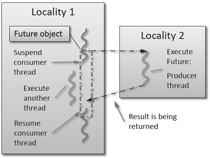
As shown in the figure below, a Future encapsulates a delayed computation. It acts as a proxy for a result initially not known, most of the time because the computation of the result has not completed yet. The Future synchronizes the access of this value by optionally suspending any HPX-threads requesting the result until the value is available. When a Future is created, it spawns a new HPX-thread (either remotely with a parcel or locally by placing it into the thread queue) which, when run, will execute the action associated with the Future. The arguments of the action are bound when the Future is created.

Figure 1. Schematic of a Future execution

Once the action has finished executing, a write operation is performed on the Future. The write operation marks the Future as completed, and optionally stores data returned by the action. When the result of the delayed computation is needed, a read operation is performed on the Future. If the Future's action hasn't completed when a read operation is performed on it, the reader HPX-thread is suspended until the Future is ready. The Future facility allows HPX to schedule work early in a program so that when the function value is needed it will already be calculated and available. We use this property in our Fibonacci example below to enable its parallel execution.

Setup

The source code for this example can be found here: fibonacci.cpp.

To compile this program, go to your HPX build directory (see Getting Started for information on configuring and building HPX) and enter:

make examples.quickstart.fibonacci

To run the program type:

./bin/fibonacci

This should print (time should be approximate):

fibonacci(10) == 55
elapsed time: 0.00186288 [s]

This run used the default settings, which calculate the tenth element of the Fibonacci sequence. To declare which Fibonacci value you want to calculate, use the --n-value option. Additionally you can use the --hpx:threads option to declare how many OS-threads you wish to use when running the program. For instance, running:

./bin/fibonacci --n-value 20 --hpx:threads 4

Will yield:

fibonacci(20) == 6765
elapsed time: 0.233827 [s]

Walkthrough

Now that you have compiled and run the code, let's look at how the code works. Since this code is written in C++, we will begin with the main() function. Here you can see that in HPX, main() is only used to initialize the runtime system. It is important to note that application-specific command line options are defined here. HPX uses Boost.Program Options for command line processing. You can see that our programs --n-value option is set by calling the add_options() method on an instance of boost::program_options::options_description. The default value of the variable is set to 10. This is why when we ran the program for the first time without using the --n-value option the program returned the 10th value of the Fibonacci sequence. The constructor argument of the description is the text that appears when a user uses the --help option to see what command line options are available. HPX_APPLICATION_STRING is a macro that expands to a string constant containing the name of the HPX application currently being compiled.

In HPX main() is used to initialize the runtime system and pass the command line arguments to the program. If you wish to add command line options to your program you would add them here using the instance of the Boost class options_description, and invoking the public member function .add_options() (see Boost Documentation or the Fibonacci Example for more details). hpx::init() calls hpx_main() after setting up HPX, which is where the logic of our program is encoded.

int main(int argc, char* argv[])
{
    // Configure application-specific options
    boost::program_options::options_description
       desc_commandline("Usage: " HPX_APPLICATION_STRING " [options]");

    desc_commandline.add_options()
        ( "n-value",
          boost::program_options::value<boost::uint64_t>()->default_value(10),
          "n value for the Fibonacci function")
        ;

    // Initialize and run HPX
    return hpx::init(desc_commandline, argc, argv);
}

The hpx::init() function in main() starts the runtime system, and invokes hpx_main() as the first HPX-thread. Below we can see that the basic program is simple. The command line option --n-value is read in, a timer (hpx::util::high_resolution_timer) is set up to record the time it takes to do the computation, the fibonacci action is invoked synchronously, and the answer is printed out.

int hpx_main(boost::program_options::variables_map& vm)
{
    // extract command line argument, i.e. fib(N)
    boost::uint64_t n = vm["n-value"].as<boost::uint64_t>();

    {
        // Keep track of the time required to execute.
        hpx::util::high_resolution_timer t;

        // Wait for fib() to return the value
        fibonacci_action fib;
        boost::uint64_t r = fib(hpx::find_here(), n);

        char const* fmt = "fibonacci(%1%) == %2%\nelapsed time: %3% [s]\n";
        std::cout << (boost::format(fmt) % n % r % t.elapsed());
    }

    return hpx::finalize(); // Handles HPX shutdown
}

Upon a closer look we see that the hpx::lcos::future<> we created is assigned the return of hpx::lcos::async<fibonacci_action>(hpx::find_here(), n). hpx::lcos::async<>() takes an action, in this case fibonacci_action, and asynchronously kicks of the computation of the action, returning a future which represents the result of the computation. But wait, what is an action? And what is this fibonacci_action? For starters, an action is a wrapper for a function. By wrapping functions, HPX can send packets of work to different processing units. These vehicles allow users to calculate work now, later, or on certain nodes. The first argument to hpx::lcos::async<>() is the location where the action should be run. In this case, we just want to run the action on the machine that we are currently on, so we use hpx::find_here(). To further understand this we turn to the code to find where fibonacci_action was defined:

// forward declaration of the Fibonacci function
boost::uint64_t fibonacci(boost::uint64_t n);

// This is to generate the required boilerplate we need for the remote
// invocation to work.
HPX_PLAIN_ACTION(fibonacci, fibonacci_action);

A plain action is the most basic form of action. Plain actions wrap simple global functions which are not associated with any particular object (we will discuss other types of actions in the Accumulator Example). In this block of code the function fibonacci() is declared. After the declaration, the function is wrapped in an action in the declaration HPX_PLAIN_ACTION. This function takes two aruments: the name of the function that is to be wrapped and the name of the action that you are creating.

This picture should now start making sense. The function fibonacci() is wrapped in an action fibonacci_action, which was spawned by hpx::lcos::async<>(), which returns a future. Now, lets look at the function fibonacci():

boost::uint64_t fibonacci(boost::uint64_t n)
{
    if (n < 2)
        return n;

    // We restrict ourselves to execute the Fibonacci function locally.
    hpx::naming::id_type const locality_id = hpx::find_here();

    // Invoking the Fibonacci algorithm twice is inefficient.
    // However, we intentionally demonstrate it this way to create some
    // heavy workload.

    fibonacci_action fib;
    hpx::future<boost::uint64_t> n1 =
        hpx::async(fib, locality_id, n - 1);
    hpx::future<boost::uint64_t> n2 =
        hpx::async(fib, locality_id, n - 2);

    return n1.get() + n2.get();   // wait for the Futures to return their values
}

This block of code is much more straightforward. First, if (n < 2), meaning n is 0 or 1, then we return 0 or 1 (recall the first element of the Fibonacci sequence is 0 and the second is 1). If n is larger than 1, then we spawn two futures, n1 and n2. Each of these futures represents an asynchronous, recursive call to fibonacci(). After we've created both futures, we wait for both of them to finish computing, and then we add them together, and return that value as our result. The recursive call tree will continue until n is equal to 0 or 1, at which point the value can be returned because it is implicitly known. When this termination condition is reached, the futures can then be added up, producing the n-th value of the Fibonacci sequence.